Critical Metrics for Digital Threads, Part 3 – Complexity

The consideration of complexity concerning digital threads is a matter of both good and bad news. The literature on digital complexity metrics is rich with detailed algorithms for graphs and software code, many already available in Python and Gremlin libraries applicable to our demonstration example. On the other hand, the relevance of these to project management issues of cost, schedule, and risk is a much more open question.

That complexity is relevant to these issues seems reasonable. The more different types of model elements and the more options for connecting them, the greater the opportunity for error and rework. The greater the number of cross-cutting connections between different subsystems, the greater the chance a small change may trigger an exponentially increasing cascade of changes all across the system model.

Many of these ideas are already expressed in graph theory and applicable to the Syndeia digital thread graph, including

• Connectivity – how many disconnected graphs (e.g., fully independent subsystems) exist? What is the average number of edges per node (e.g., relations per artifact)?
• Tree Structure and Cycles – is there a single path between any two nodes (acyclic graph)?
• Cliques and Clusters – are there groups of nodes that all link to each other?
• Centrality – which nodes (e.g., artifacts) are connected to the most other nodes?

Many necessary algorithms are already available in the open-source Tinkerpop Gremlin query language and immediately available to Syndeia users.

If we make an analogy between a digital thread and software code, the digital work product of systems engineers vs. software engineers, there are metrics from the software world we can seek to apply:

• Decision Points (Cyclomatic Complexity) – at how many points in the workflow must the system engineers make a choice, and how many options are possible for each alternative?
• Halstead’s Metric – how many unique types of artifacts and relations ( analogous to operands and operators) are there, and what is the frequency of their use?
• Time Complexity – how many different types of artifacts are being added to the digital thread simultaneously (parallel vs. serial processes)?

While robust and well-developed, these concepts are generally unfamiliar to working systems engineers and project managers. We will approach the topic with simpler questions to illustrate the raw data available from our digital thread example and lay the basis for more complex metrics.

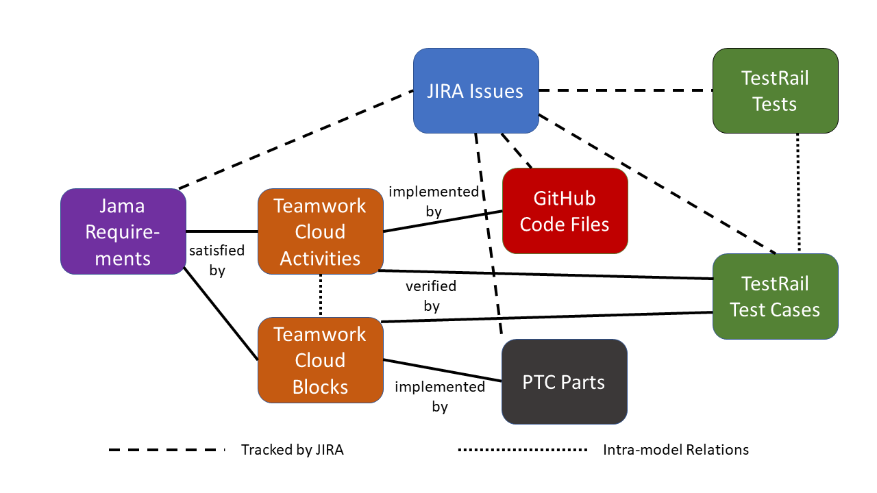
Figure 1 Sample Schema

As discussed in Part 2 of this series, our metrics are calculated from a sample model, an Unmanned Ground Vehicle (UGV02), as shown in Figure 1.

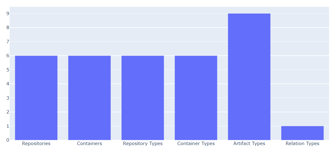
Figure 2 Project Node and Node Type Counts

The simplest measure of project complexity is the number of high-level elements (repositories and containers) and element types participating in this digital thread. These are shown in Figure 2, taken from a Jupyter notebook using, as are most subsequent figures, the plotly and pandas visualization libraries available for Python. These values represent complexity by indicating the number of first-order choices available each time a new relation is added to the digital thread.

The first four columns all have the same value, 6, indicating six repositories participating in the digital thread, each of a different type, each with one participating container or project of a unique type. While this may represent a common, relatively simple scenario, it is not the only possibility. Multiple repositories of the same type or various containers within one repository participating in the digital thread may exist.  In this example, there is only one relation type, an unspecialized reference connection, but more specialized relation types may be created and used. All of the factors will increase the complexity of the thread.

Figure 3.a # Connected Artifacts by Repository

Figure3.b Mean Connectivity by Repository

The pie chart in Figure 3.a reports the number of artifacts in each of the six repositories that are part of the digital thread for a particular project. This does not include all the artifacts in each repository, only those connected in this specific thread. The complexity of this thread is indicated by the number of different repositories involved and the total number of artifacts, given that the scale of the thread is one aspect of complexity.

Figure 3. b extends this approach to calculating the mean connectivity, i.e., the average number of connections per artifact for each repository. This would measure centrality, which types of artifacts are most heavily connected. Note that mean connectivity cannot be less than one; nodes that have zero inter-model connections are not part of this digital thread.

The two metrics plotted in the pie charts appear strongly correlated, at least at this point in the digital thread development. Jama requirements and JIRA issues are most fully embedded in the thread, both in terms of number and connectivity. Given the high centrality for JIRA suggested by the schema in Figure 3, we might expect this correlation to decrease as the thread develops.

In the next post in this blog series, we will explore measures of Activity, the rate at which the digital thread is extended, with a breakdown of activity by the repository involved.

For more blogs in the series:

• Critical Metrics for Digital Threads, Part 1 
• Critical Metrics for Digital Threads, Part 2
• Critical Metrics for Digital Threads, Part 3 (This Part)
• Critical Metrics for Digital Threads, Part 4
• Critical Metrics for Digital Threads, Part 5 
• Critical Metrics for Digital Threads, Part 6 
• Critical Metrics for Digital Threads, Part 7
• Critical Metrics for Digital Threads, Part 8 
• Critical Metrics for Digital Threads, Part 9

Tweet